Discounted Cash Flow Models (DCF): Guide and Examples
Discounted cash flow (DCF) analysis is a method used in corporate finance and valuation to estimate the attractiveness of an investment opportunity. DCF analysis uses future free cash flow projections and discounts them to arrive at a present value estimate, which is used to evaluate the potential for investment.
Article Contents
Key Takeaways
| Key Takeaway | Description |
|---|---|
| Definition of DCF | DCF analysis is a method used to estimate the value of an investment opportunity by discounting future free cash flow projections to their present value. |
| Structure of a DCF Model |
|
| DCF Calculation Steps |
|
| Advantages of DCF |
|
| Disadvantages of DCF |
|
| Key Inputs |
|
| Applications in Corporate Finance |
|
WHAT IS A DISCOUNTED CASH FLOW ANALYSIS?
A DCF analysis values a project, company, or asset using the concept of the time value of money. All future cash flows are estimated and discounted to give their present values (PVs) – the sum of all future cash flows, both incoming and outgoing, is the net present value (NPV), which is taken as the value or price of the cash flows in question.
Using DCF analysis brings future cash flows back to today’s dollars or euros using a discount rate, which captures both the time value of money and investment risk. The time value of money means that money available immediately is worth more than the same amount in the future due to its potential earning capacity.
The discount rate represents the investment’s cost of capital or the minimum acceptable rate of return.
The term “DCF analysis” usually is used in the context of valuing shares or companies. The price of a bond is the discounted value of the bonds cashflows to maturity, discounted at the bond yield. Traders and investors don’t tend to talk about DCF though in this context, they just talk about bond prices and yields.
Structure Of A DCF Model
A DCF model is structured in the following way:
- Forecast period: A finite period of time, usually 5-10 years, for which future cash flows are estimated.
- Terminal value: An estimate of the value of cash flows beyond the forecast period.
- Discount rate: The annual required rate of return, which reflects the riskiness of estimated cash flows.
- Present value: The discounted value of the forecasted cash flows and terminal value.
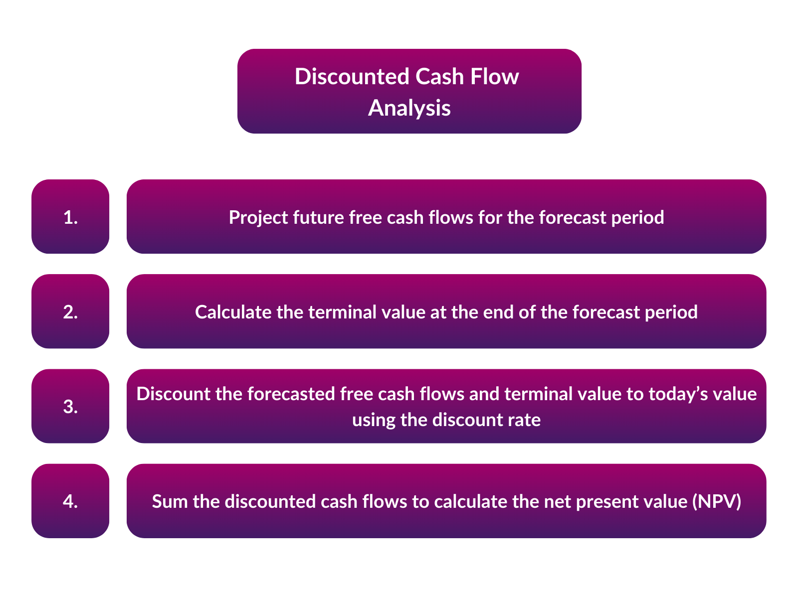
The steps for building a DCF model are:
- Project future free cash flows for the forecast period.
- Calculate the terminal value at the end of the forecast period.
- Discount the forecasted free cash flows and terminal value to today’s value using the discount rate.
- Sum the discounted cash flows to calculate the net present value (NPV).
How to Calculate a DCF MODEL IN EXCEL
How to calculate a DCF model in Excel
Here are the steps to calculate a DCF model in Excel:
- Create a forecast of the free cash flows in the forecast period (e.g. 5 years).
- Free cash flow = EBITDA – the increase/plus the decrease in working capital – capital expenditures – notional tax on EBIT.
- The tax rate used is the effective cash tax rate paid by the company.
- Add a column for terminal value after the forecast period. The terminal value can be calculated treating the cash flows after the explicit forecast as a growing perpetuity. The formula for that perpetuity value after 5 years is calculated using the formula:
- Terminal Value = Final Year Cash Flow x (1 + Growth Rate) / (Discount Rate – Growth Rate)
- Make a row for the discount factor based on the discount rate chosen.
- Discount Factor = Discount Factor = 1 / (1 + Discount Rate)^Year
- Discount each cash flow by multiplying it with the discount factor. The discount used is typically the weighted average cost of capital or “WACC”. This is the weighted average after tax costs od debt and equity of the company. This might be as low as 6-8% for a large “blue-chip” listed company. It may be double or triple this amount for a risky venture.
- A common mistake here is to discount the terminal value as though it is received in year 6. It is the value at year 5, i.e. 1 year before the first cashflow in the growing perpetuity.
- Sum all the discounted cash flows to get the present value. In the case of a company this gives us the enterprise value or “EV”. Subtract the net debt to give a valuation for the equity of the business. In the case of a listed company, divide the equity value into the number of shares in issue to give an implied per-share value.
Advantages and Disadvantages of Discounted Cash Flow Analysis
Advantages of DCF:
- Considers the time value of money – Early cash flows are worth more than later ones.
- Cash flow-based – Focus on projected cash flows rather than net income.
- Flexibility – Various scenarios can be modelled by adjusting inputs.
- Helps identify viable investments – Positive NPV indicates value creation, shares priced below the DCF implied value likewise indicate a cheap stock.
Disadvantages of DCF:
- Projections may not be accurate – Garbage in, garbage out.
- Does not account for externalities or strategic considerations.
- Requires choosing a discount rate – Can be subjective.
- Terminal value relies on estimates and assumptions.
- Time-consuming and relies on many inputs.
Common Challenges When Performing a DCF Analysis
Determining an appropriate discount rate is often cited as one of the most complex aspects of DCF analysis. The discount rate is essentially the cost of capital, which reflects the expected return required by investors. Determining this rate involves:
- Risk-Free Rate: This is usually the yield on government bonds and represents the long-term return expected from a completely risk-free investment.
- Beta: This is the relative volatility of a stock versus the market. This is used as the measure of how much riskier the investment is compared to the broader market. Beta is used to adjust the discount rate to reflect risk.
- Market Risk Premium: Calculated as the expected return of the market minus the risk-free rate, it represents the additional average long-term return required by investors for taking on the extra risk of investing in the market.
- After-tax Cost of Debt: Represents the yield at which the company would expect to pay on new debt raised today. This is often synthesised by looking at current government bond yields and applying an appropriate credit spread. TO give the after-tax cost, the debt yield is discounted at the tax rate. So the formula is After tax cost of debt (Kd)= Yield*(1-tax rate).
A basic formula to calculate the discount rate (for use in DCF) might be:
Ke = Cost of Equity = Risk-Free Rate + (Beta x Market Risk Premium)
The Cost of Capital (WACC) is given by the formula:
WACC = Equity/EV*Ke +Net debt/EV*Kd
Accurately estimating future cash flows is also complex. Analysts must make assumptions about future performance and growth rates. An alternative to the perpetuity method for Terminal value is to use an exit multiple after 5 years. This again is subjective. All these different factors can significantly impact the DCF valuation. It’s beneficial to employ various scenarios and sensitivity analyses to understand the range of possible outcomes and intrinsic risks.
As an equity analyst, rather than making our own assumptions, we can use a DCF model to ask the question “what has to be true for the current share price to be correct?” This can give us a very useful insight into the cheapness/expensiveness of a share.
Applications of DCF in Corporate Finance
DCF has several applications in corporate finance:
- Investment Decision Making – Assess capital budgeting projects like expanding operations. Positive NPV indicates projects to accept.
- Mergers and Acquisitions – Value takeover targets and assess synergies.
- Stock Valuation – Value a company’s shares based on projected dividends / free cash flows to equity.
- Capital Structure – Evaluate impact of debt financing versus equity financing on the value of a business.
- Project and Company Valuation – Value investment projects, entire companies, or assets based on free cash flows.
DCF provides a forward-looking estimate of value based on expected cash flows. By estimating future cash flows and risk-adjusting the valuation through the discount rate, DCF helps guide corporate finance strategy.
Exercises and Examples for DCF
Example 1:
A company expects free cash flows of $100,000 for the next 5 years, and the discount rate is 10%. What is the net present value (NPV)?
Solution:
- Year 1: $100,000 / (1 + 10%)^1 = $90,909
- Year 2: $100,000 / (1 + 10%)^2 = $82,644
- Year 3: $100,000 / (1 + 10%)^3 = $75,131
- Year 4: $100,000 / (1 + 10%)^4 = $68,301
- Year 5: $100,000 / (1 + 10%)^5 = $62,092
- NPV = $90,909 + $82,645 + $75,131 + $68,301 + $62,092 = $379,077
Example 2:
A project requires an initial investment of $500,000 and is expected to create free cash flows of $150,000 per year for 4 years. If the cost of capital is 12%, what is the project NPV? Should it be accepted?
Solution:
- Year 0: -$500,000
- Year 1: $150,000 / (1 + 12%)^1 = $133,929
- Year 2: $150,000 / (1 + 12%)^2 = $119,420
- Year 3: $150,000 / (1 + 12%)^3 = $106,386
- Year 4: $150,000 / (1 + 12%)^4 = $94,804
- NPV = -$500,000 + $133,929 + $119,420 + $106,767 + $95,328 = -$44,398
Since the NPV is negative, the project value is less than the initial investment. Therefore, it should be rejected.
In summary, discounted cash flow analysis is a pivotal valuation method in corporate finance, enabling companies to assess investments and projects based on their anticipated cash flow potential. By forecasting free cash flows, calculating terminal value, discounting to present value, and determining NPV, DCF offers a means to compare capital budgeting decisions and decide whether they create shareholder value. While DCF does depend on projections and comes with its own set of challenges, particularly around determining appropriate discount rates and future cash flows, it remains a widely utilized and insightful method for corporate finance strategy and valuation.
DCF FAQs

An experienced finance and training professional and Co-Founder of Capital City Training Ltd, Greg has a demonstrated history of working in the financial services sector and has a passion for sharing his knowledge and skills throughout the financial services sector. He has been partnering financial and corporate clients in designing and delivering applied financial programs that make an impact on business outcomes. Greg is skilled in accounting & financial analysis, derivatives and risk management, financial modelling, business valuation and corporate finance and has worked with the worlds leading financial institutions. A strong business development professional and a qualified accountant (ICAEW member), CFA Charterholder and Associate Member of the Association of Corporate Treasurers in the UK (ACT).